In this project you will use numpy arrays.
For a brief example using them click
HERE
 .
.
To plot the data I suggest you use the pyplot or related modules.
matplotlib.pyplot
(documentation and examples)
For more matplotlib.pyplot examples click
HERE
.
Project Outline
1. Define a compound signal
made from sine and cosine waves
with differing frequencies.
2. Create an array of sampling
monotonically increasing times. This will be used
to sample the compound signal.
(This is is a sample of the compound
signal in the time domain.)
3. Plot the sample values.
This is the signal in the Time Domain.
(See the example below.)
4. Using the time sample array, take samples of
the compound signal and save them in an array.
5. Compute a Fast Fourier Transform (FFT) of the
of the time based sample array.
(use the Python library shown in the code example below.)
6. Plot the frequency FFT values.
- create an array of frequency steps
than covers the range of frequencies.
- Plot the frequency steps vs
the FFT frequencies values.
This is the compound signal in the Frequency Domain.
(See the example below.)
7. Plot an expanded version of the plot in #6.
Use the first 1/2 of the each array in #6.
(Make sure there in the same number
of elements is in each array.)
This is the signal in the Frequency Domain.
(See the example below.)
Project #1
Apply the following steps using the initial data.
signal1 frequency = 100
signal2 frequency = 200
signal3 frequency = 50
sample frequency = 2000
sample time step = 0.0005
sample freq step = 10.0
Step #1 - Define Parameters/Variables for the Program
| variable | Description |
|---|
| sigfreq | signal frequency (hz)
(base frequency for sampling) |
| samfreq | sampling frequency (hz) |
| timstep | time interval between two samples
1/samfreq |
| n | number of samples
int(10 * samfreq/sigfreq) |
| freqstep | frequency intervals
between two samples
samfreq/n |
samples : 0 - 199 (samples)
time step : 0.0005 (sec)
sample time: first = 0.0 last = 0.0995
Step #2 - FTT of Signal Sample
# Note: in this example all of the signals
# have the same magnitude (1.0)
import numpy as np
# ---- signal 1 - sine function - frequency 100
# ---- double the signals magnitude (multiply by 2)
# ---- y1 is a numpy array
y1 = np.sin(2 * np.pi * sigfreq * t)
# ---- signal 2 - sine function - frequency 200
# ---- double the signals magnitude (multiply by 2)
# ---- y2 is a numpy array
y2 = np.sin(2 * np.pi * sigfreq * t * 2)
# ---- signal 3 - sine function - frequency 50
# ---- double the signals magnitude (multiply by 2)
# ---- y3 is a numpy array
y3 = np.sin(2 * np.pi * sigfreq * t * 0.5)
# ---- combine the signals (y is a numpy array)
y = y1 + y2 + y3
# ---- perform FFT on samples of the combine signal
# ---- x is a numpy array of complex numbers
# ---- convert FFT results to absolute values
x = np.fft.fft(y)
# ---- normalize the absolute values
xabs = np.abs(x)/n
Step #3 - Create Arrays For Plotting
# ---- array of sampling times (numpy array)
# ---- used for time domain plots
t = np.linspace(0,(n-1)*timstep,n)
# ---- array of sampling frequencies (numpy array)
# ---- used for frequency domain plots
f = np.linspace(0,(n-1)*freqstep,n)
Step #4 - Plot the Data For Analysis
Plot the data using subplots. Make it look like the
example below.
plot t,y # full time range
plot f,xabs # full frequency range
# Note: x1 and x2 - correct DC (frequency 0) magnitude by
# dividing by 2 because they are multiplied by 2
x2 = 2 * xabs[0:int(n/2+1)] # magnify X 2
x2[0] = x2[0]/2 # correct frequency 0
plot f/2,x2 # 1/2 frequency range
x4 = 2 * xabs[0:int(n/2+1)] # magnify X 2
x4[0] = x4[0]/2 # correct frequency 0
plot f/4,x4 # 1/4 frequency range
What frequencies did you find?
Did you find the original frequencies?
Intermediate Arrays, etc.
t array len(t)=200 t[0]=0.0 t[-1]=0.0995
f array len(f)=200 f[0]=0.0 f[-1]=1990.0
y1 array len(y1)=200 y1[0]=0.0 y1[-1]=-0.309017
y2 array len(y2)=200 y2[0]=0.0 y2[-1]=-0.587785
y3 array len(y3)=200 y3[0]=0.0 y3[-1]=-0.156434
y array len(y) =200 y[0]=0.0 y[-1]=-1.053237
x array len(x)=200 x[0]=-0.000000+0.000000j x[-1]=-0.000000-0.000000j
x_abs array len(x_abs)=200 x_abs[0]=0.000000 x_abs[-1]=0.000000
Plots
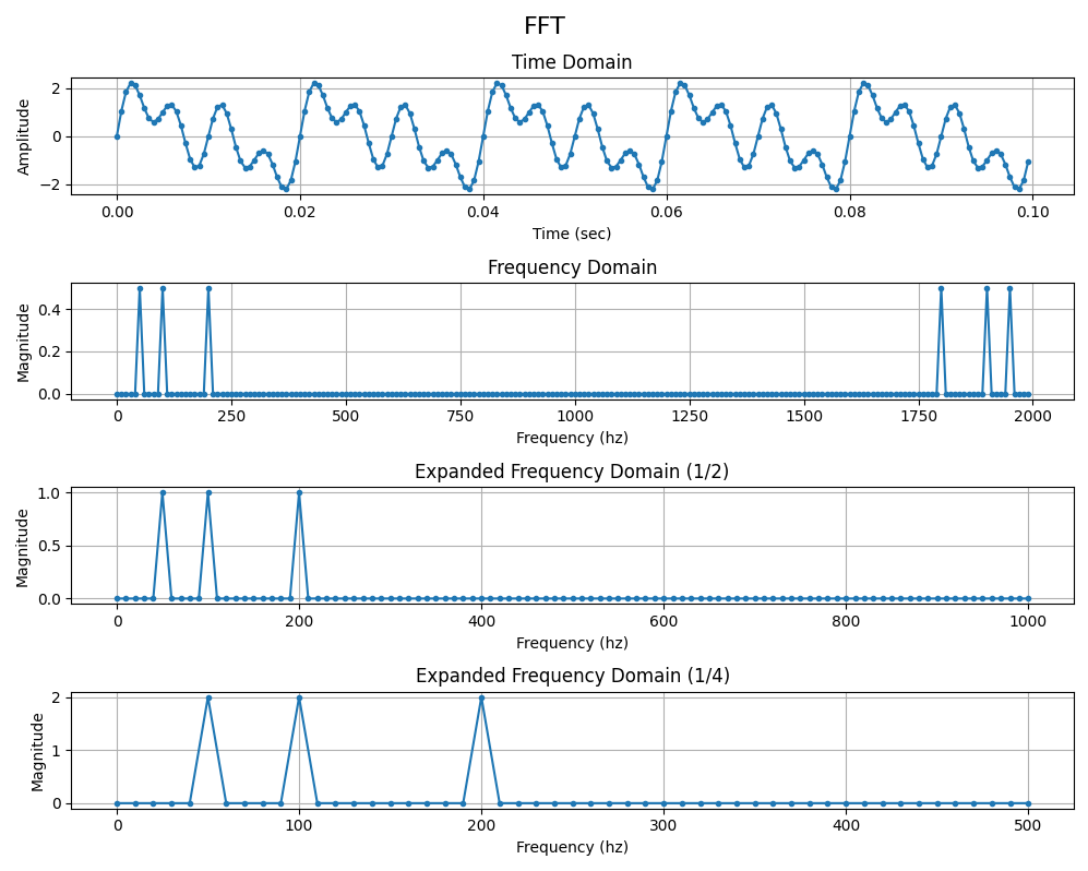
Plot created using 4 sublplots.