Introduction
Wave, propagation of disturbances from place to place in a regular and organized way. Most familiar are surface waves that travel on water, but sound, light, and the motion of subatomic particles all exhibit wavelike properties. (www.britannica.com)
Some physical phenomenon can be described by wave equations. For example radio waves or ocean waves. When two or more of these waves meet interesting things happen.
Waves can be described using cycles per second, hertz, wave length, etc.
This project combines waves and displays the form of the combined waves. Users can "play" with the characteristics of the waves and see what develops.
Hertz are the SI unit of frequency equal to one cycle per second. Usually the frequency of radio transmissions or computer clock speed.
- 1hz or 1Hz is 1 (one) cycle per second.
- 1KHz is 1,000 (1 thousand) cycles per second.
- 1MHz is 1,000,000 (1 million) cycles per second.
- 1GHz is 1,000,000,000 (1 billion) cycles per second.
Note: The International System of Units (SI), commonly known as the metric system, is the international standard for measurement.
Sine, Cosine Wave
Frequency is 100hz.
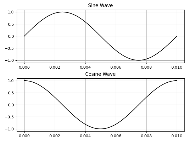
How are sine waves related to circles? (YouTube)
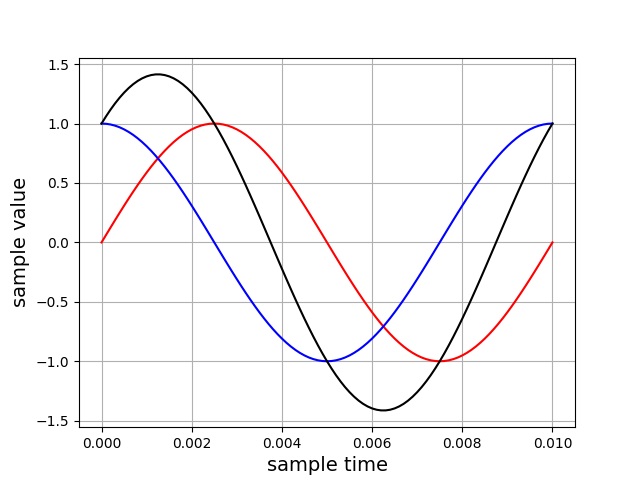
Example #1
This plot shows the combining of a sine and cosine waves.
- Both waves have the same start time (0.0)
- Sine wave's frequency is 100hz
- Cosine wave's frequency is 100hz
- Black is the combined waves
- Red is the sine wave
- Blue is the cosine wave
- Sine and cosine waves vary between -1 and +1
- The sample range is 0.0 to 0.01 seconds
- The sample size is 100
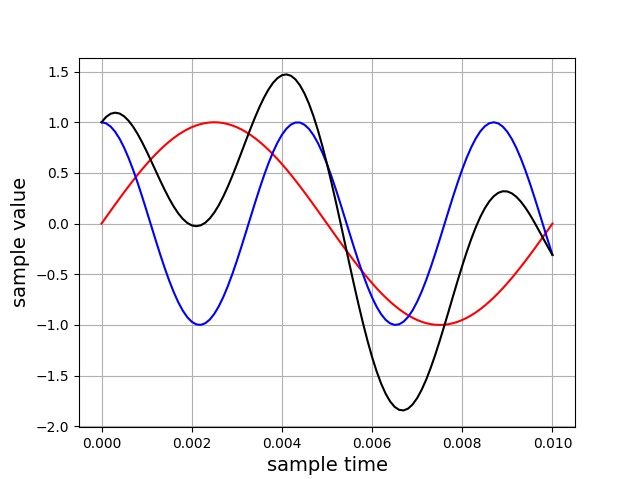
Example #2
This plot shows the combining of a sine and cosine waves.
- Both waves have the same start time (0.0)
- Sine wave's frequency is 100hz
- Cosine wave's frequency is 230hz
- Black is the combined waves
- Red is the sine wave
- Blue is the cosine wave
- Sine and cosine waves vary between -1 and +1
- The sample range is 0.0 to 0.01 seconds
- The sample size is 100
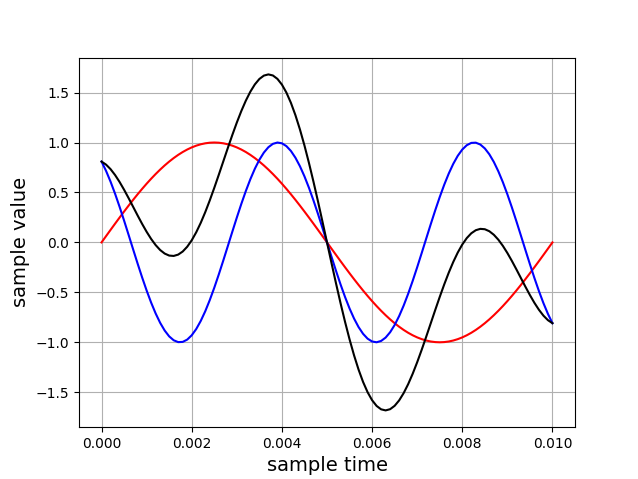
Example #3
This plot shows the combining of a sine and cosine waves.
- Sine wave start time is 0.0
- Cosine wave start time is -0.43
- Sine wave's frequency is 100hz
- Cosine wave's frequency is 230hz
- Black is the combined waves
- Red is the sine wave
- Blue is the cosine wave
- Sine and cosine waves vary between -1 and +1
- The sample range is 0.0 to 0.01 seconds
- The sample size is 100
Project #1
Write a program to demonstrate combining the two waves described in example #1 above.
To plot the data I suggest you use the pyplot or related modules.
matplotlib.pyplot (documentation and examples)
For more examples click
HERE.
Note: To combine waves the sample should be the same start, end, and size.
Project #2
Write an interactive program that allows a users to do the following kinds of things.
- Select various sine or cosine waves (different frequencies, ...)
- Plot the combined wave, change parameters, and plot again
- Plot individual waves and the combined wave
- Combine two or more waves (multiple sine and cosine waves?)
- Change the frequency of each wave
- Change the star time of each wave
- Change the sample start and end time
Sample start time < sample end time - Change the sample size (sample size > 0)
- Scale the plot's Y values (-100 to +100) (-235 to +235) ... ?
use the maximum wave value/magnitude/strength (see max function)
Project #3
Modify Program #2. Add other wave functions. let the user select the functions to use. Functions like ...
- additional sine and cosine waves
(different frequencies?) (different start times?) - square waves
See numpy.step() and pyplot.step() - triangle waves
- sawtooth waves
- ....
Note: Wave functions must be continuous.
Project #4
Add a (one) serpentine curve to Project #2.
Click HERE
 for serpentine curve code.
Some Example Code to Get You Started
FYI
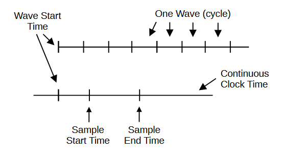
Picking the wave frequency,
and the sample start and end times can be tricky.
This diagram will help you visualize the problem.
Waves Forms
Note: A sinusoidal wave is a periodic wave whose waveform (shape) is the trigonometric sine function. (Wikipedia)
 # ---- wave value function
def value(hz,t):
freq = hz
period = 1/freq
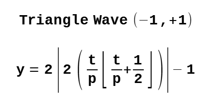
v = 2 * abs(2 * (t/period - math.floor((t/period)+(1/2)))) - 1
return v
# ---- examples test parameters
hz = 1.0 # frequency
sstart = 0.0 # sample start time
send = 2.0 # sample end time
ssize = 1000 # sample size
# ---- wave value function
def value(hz,t):
freq = hz
period = 1/freq
v = 2 * abs(2 * (t/period - math.floor((t/period)+(1/2)))) - 1
return v
# ---- examples test parameters
hz = 1.0 # frequency
sstart = 0.0 # sample start time
send = 2.0 # sample end time
ssize = 1000 # sample size
 # ---- wave value function
def value(hz,t):
freq = hz
period = 1/freq
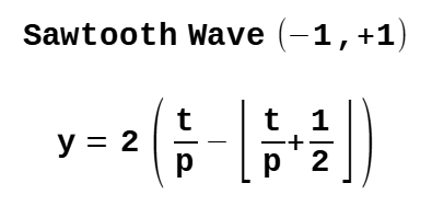
v = 2 * (t/period - math.floor((1/2) + (t/period)))
return v
# ---- examples test parameters
hz = 1.0 # frequency
sstart = 0.0 # sample start time
send = 2.0 # sample end time
ssize = 1000 # sample size
# ---- wave value function
def value(hz,t):
freq = hz
period = 1/freq
v = 2 * (t/period - math.floor((1/2) + (t/period)))
return v
# ---- examples test parameters
hz = 1.0 # frequency
sstart = 0.0 # sample start time
send = 2.0 # sample end time
ssize = 1000 # sample size
 # ---- sign function
def sgn(x):
if x > 0: return 1
if x == 0: return 0
return -1
# ---- wave value function
def value(hz,t):
freq = hz
rad = 2.0*math.pi*freq*t
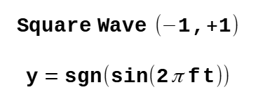
v = sgn(math.sin(rad))
return v
# ---- examples test parameters
hz = 1.0 # frequency
sstart = 0.0 # sample start time
send = 2.0 # sample end time
ssize = 1000 # sample size
# ---- sign function
def sgn(x):
if x > 0: return 1
if x == 0: return 0
return -1
# ---- wave value function
def value(hz,t):
freq = hz
rad = 2.0*math.pi*freq*t
v = sgn(math.sin(rad))
return v
# ---- examples test parameters
hz = 1.0 # frequency
sstart = 0.0 # sample start time
send = 2.0 # sample end time
ssize = 1000 # sample size